How We Load 17.7 Billion Readings in One Second

Summary

A plant's historian holds years of SCADA and DCS readings, stored as data streams called tags. A typical refinery can have 200,000 to 500,000 tags, each updating anywhere from once a day to 100 times a second. At one reading a second, 200,000 tags write about 17.3 billion readings a day.

‍

For decades, the historian's user was a person pulling a handful of trends at a time: build the chart, wait, export, clean. Now the users are AI agents, and they should not inherit that friction. They are cheap enough to run many at once, 24/7, on high-value use cases such as anomaly detection, alarm troubleshooting, and production planning. Each one needs deep history, fast, to run as many what-if checks as conditions call for.

‍

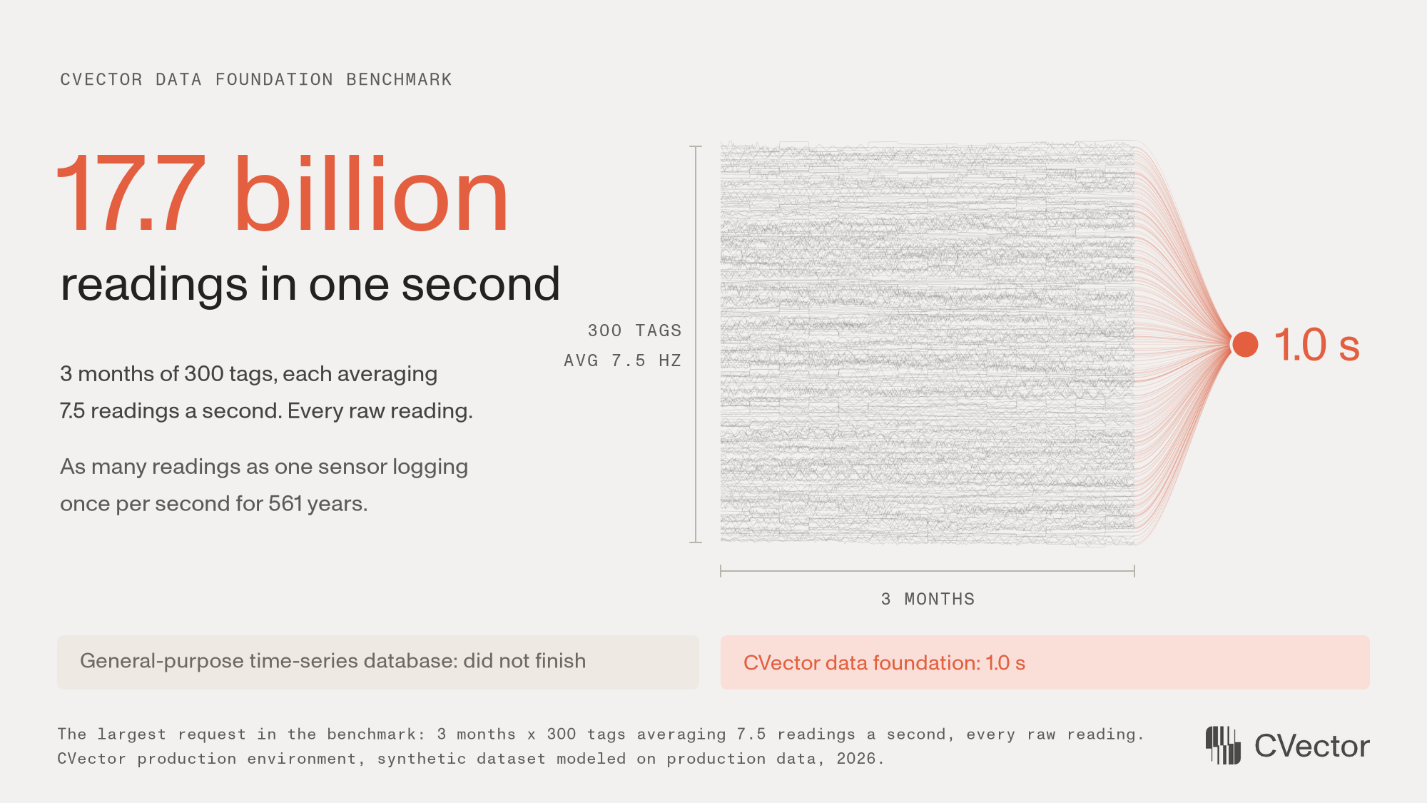
Our benchmark tests one such request: three months of history for 300 tags averaging about 7.5 readings a second, or 17.7 billion readings. An agent replays that much history to help a gas plant planner decide whether to keep recovering ethane when power prices jump on a hot afternoon.

‍

Our previous architecture could not serve that request. We used hosted TimescaleDB, the strongest time-series database we evaluated, and pushed it with continuous aggregates and bigger servers. Most month-long requests still timed out, and loads began failing at 25 simultaneous readers. Timescale is a good database, but the use cases had shifted.

‍

Working with plant data has been in CVector's DNA from the start. So we built our own data foundation, with one goal: any slice of history, at any detail, in about a second, for every agent. The results:

• All 17.7 billion raw readings from three months of 300 tags load in 1 second. The old time-series database timed out and never finished.
• New readings reach CVector's live charts in about 0.1 seconds, instead of 5.3 to 11 seconds.
• With 50 simultaneous readers, 100% of loads succeeded. On the old time-series database, 45% failed.

An hour of history for 300 tags now loads in 1.5s instead of 371s. Each agent can do about 250 times more of that work, and at least twice as many agents can run at once. So plants can test every what-if case in parallel, and operators can focus on the highest dollar-value decisions.

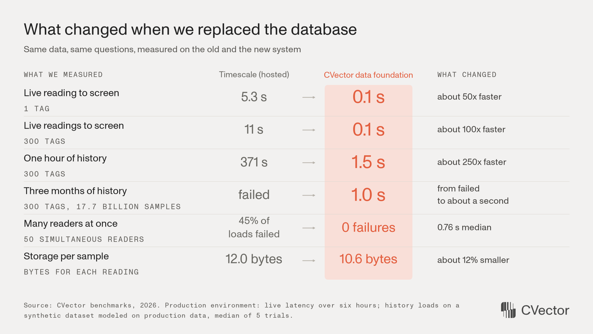
Three months of 300 tags went from failed to 1.0 s.

‍

A good database, now with a different job

Time-series databases have long been pitched as modern replacements for control-system historians such as AVEVA PI. We evaluated InfluxDB, QuestDB, DuckDB, and others. Timescale was the most performant option with SQL, the standard database language with most support, so we started on its hosted cloud service.

‍

As agents took on more of the reading, four problems kept coming up:

• Rates. Timescale works best when tuned to each tag's reporting rate. Our tens of thousands of tags report at rates we cannot know in advance, and they change without notice.
• Question size. Large ad hoc queries ran out of memory, and agents lost time rewriting them.
• Bursts. Agent work comes in bursts at any given time. The database slowed from 10 simultaneous readers across all customers and began failing at 25.
• Access rules. Its access controls did not fit our other data sources, and its permission model was not robust enough for the critical infrastructure customers we serve.

We tested various continuous aggregates sizes and options. We moved to larger servers more than once. Performance and cost simply didn't scale up and failed requests typically timed out.

‍

Timescale is a good database for many workloads, but it no longer fits our needs.

‍

Cheaper intelligence unlocks new workloads

Our workload changed as agent intelligence got cheap. In our last post, GPT-5.4 with low reasoning in fast mode had the highest pass rate on time-critical plant cases: 96.8%, at an estimated $0.371 per case.

‍

We believe those numbers show that model intelligence is being commoditized. Andreessen Horowitz and Epoch AI find the price of a given level of capability falling about tenfold a year or faster. Cheaper intelligence makes running many agents viable and cost-effective.

‍

Whenever a power price, weather forecast, or policy changes, each agent can run a what-if scenario and recalculate the plan, showing the effect on margin, schedule, and operating decisions. That adds up to a new order of magnitude in workload.

‍

For data-heavy questions, the slow and expensive part is no longer the reasoning. It is accessing the data, knowledge, and context.

‍

So the question becomes: how do you build a data layer that serves many agents making many parallel queries, running as many what-if cases as conditions demand?

‍

Designing the data foundation

We designed for that workload with two paths. A streaming channel pushes each new reading to live charts in about 0.1 seconds. A lakehouse keeps every raw reading as files that agents read directly, ready within about a second. Each of the four problems has a matching answer:

• Rates. We store every reading as it arrives, plus each tag's latest value at every minute mark, so no tag needs tuning.
• Question size. Each question brings its own computing, so large ones finish in about a second.
• Bursts. Storage and computing scale separately, so more readers do not mean a longer line.
• Access rules. Every source looks like files to an agent, under one set of rules.

The data foundation has run in production since spring 2026 across our critical infrastructure deployments, and we saw a new pattern emerge with the data friction removed for both humans and agents.

‍

What we measured

Start with live data. On the old database, a new reading was buffered, stored, and then picked up by the next poll and query. Streaming skips all three steps.

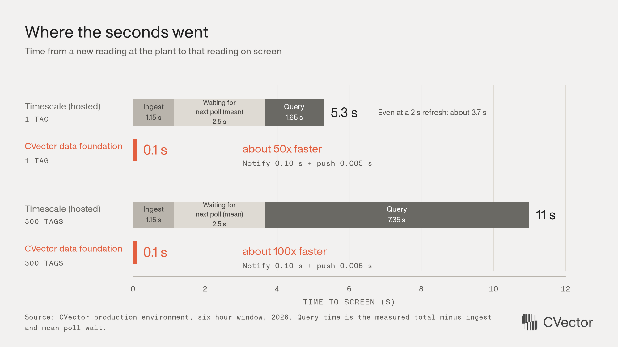
The old database stacks three delays; the data foundation's push barely shows.

‍

On our servers, a typical new reading is ready in 104 milliseconds, down from 1,151.

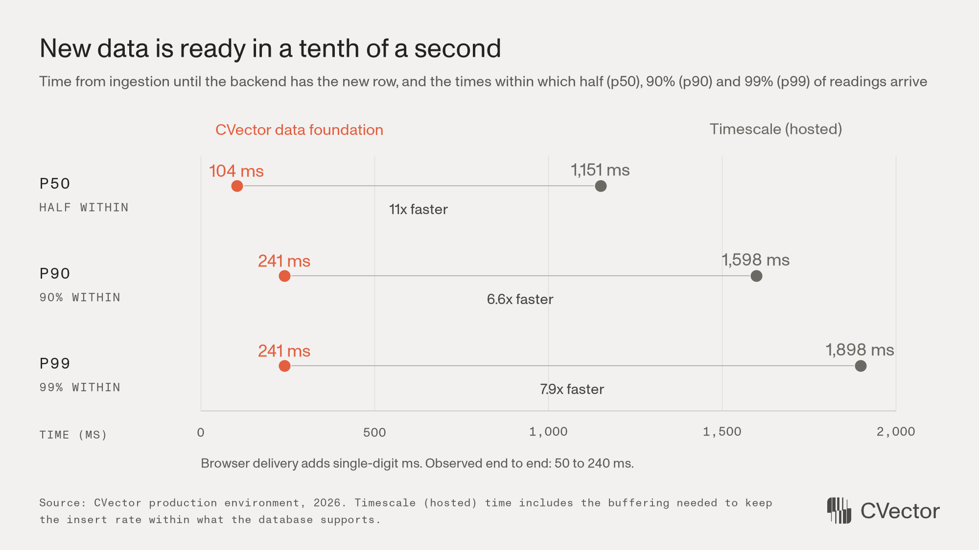
Nearly every data foundation reading arrives sooner than the old database's typical one.

‍

Next, loading historical data. Both systems ran the same 16 requests in our production environment, on a synthetic dataset modeled on real production data quality and volume. The old database took 371 seconds for an hour of 300 tags. Of the eight requests covering a month or more, it finished one: a single tag, in 129 seconds. The data foundation loaded the largest, all 17.7 billion raw readings, in 1.0 second.

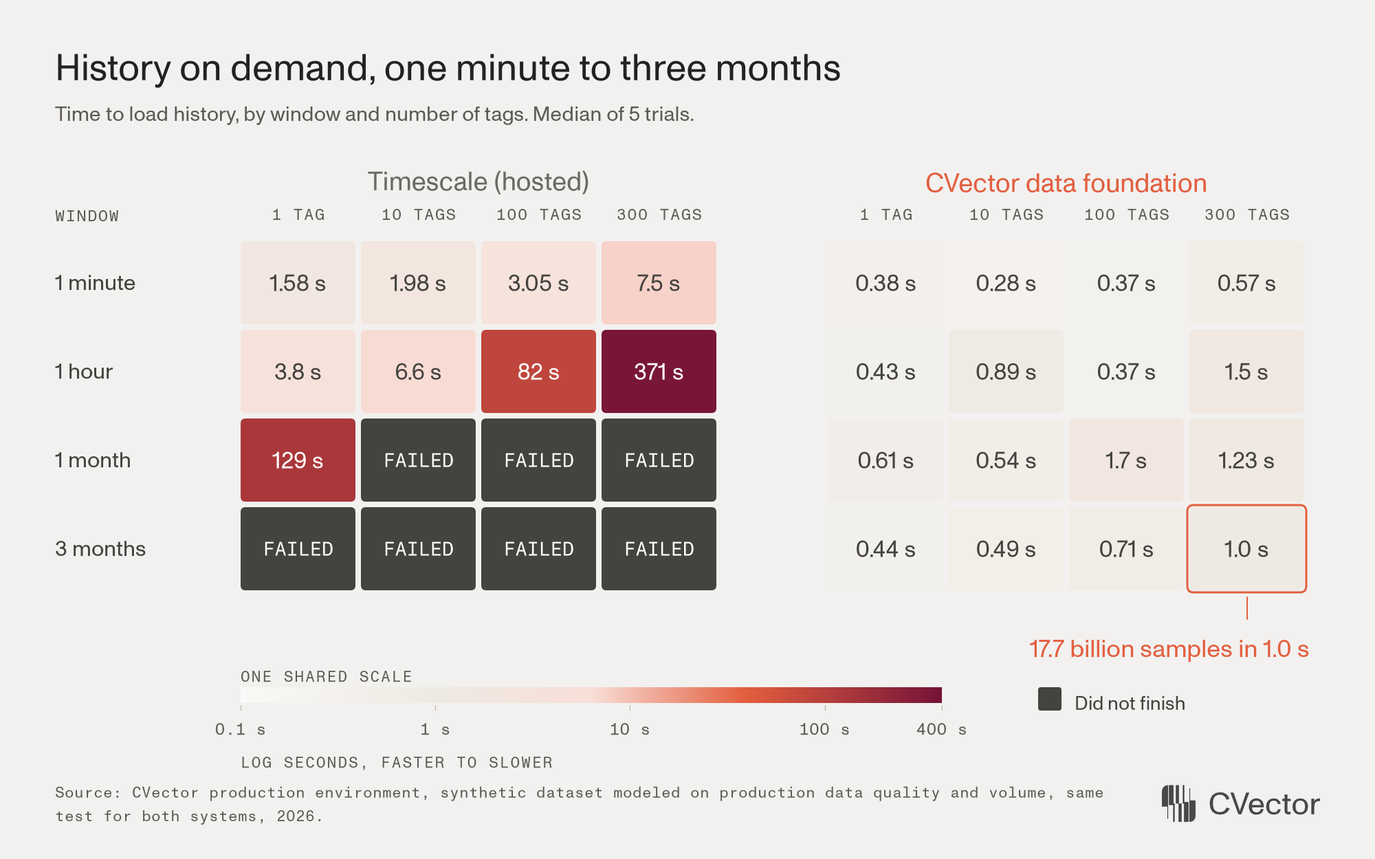
Left, times climb, then fail; right, all finish within two seconds.

‍

In CVector's data foundation, it also stores each reading in 10.6 bytes instead of 12.0, about 12% less.

Finally, many readers at once. In a load test, up to 50 simultaneous readers loaded charts. The data foundation's median load time fell to 0.76 seconds, while the old database's rose to 14.9 seconds.

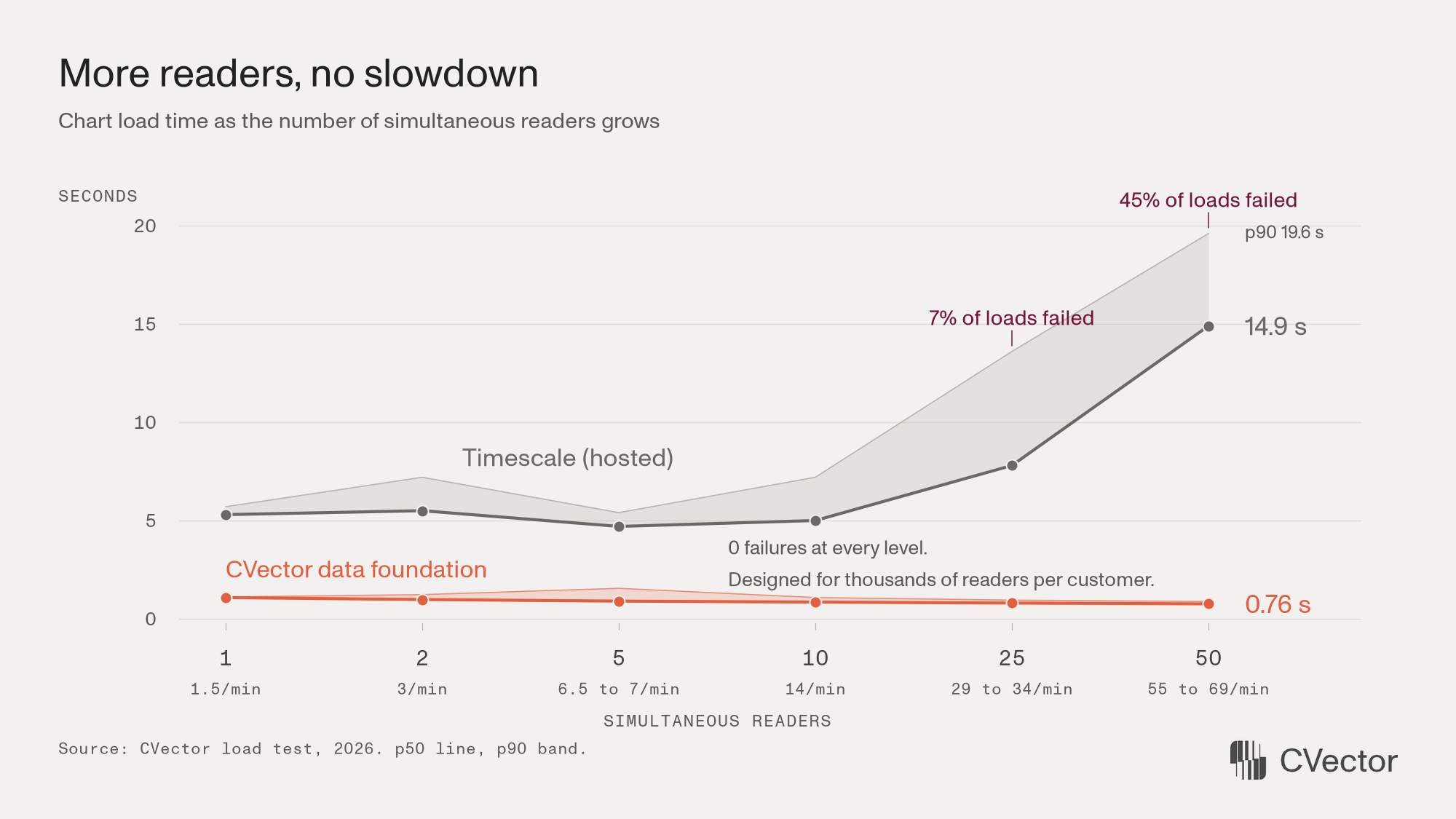
The data foundation stays flat; the old database starts failing at 25 readers.

‍

We designed the data foundation for several thousand simultaneous readers per customer. Fifty is the most we measured in this benchmark.

‍

What this makes possible

To put 17.7 billion readings in human terms: one sensor logging every second would need 561 years to collect them, starting in 1465. The old Timescale setup could only have answered in pieces. For illustration, 900 month-long, single-tag requests at the measured 129 seconds each, run back to back, would take about 32 hours.

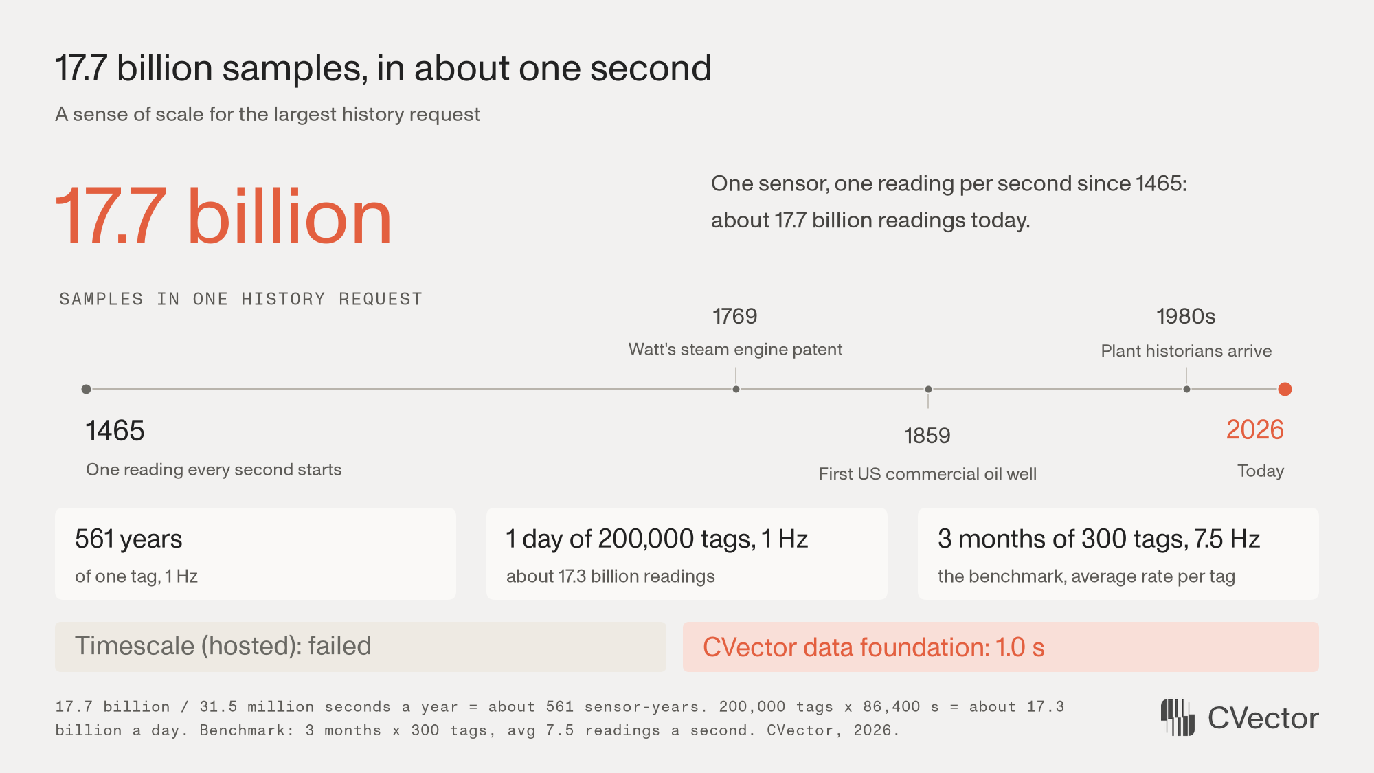
A single sensor would have had to start in 1465.

‍

Some agents compare every compressor with months of normal behavior to catch anomalies early. Some trace every tag around an outage to find what changed first. Some check all tags for gaps, flatlines, and stuck transmitters, so no answer rests on bad data. Some search hundreds of tags across seasons for correlations. Others join OT data, the readings from control systems, with power, gas, and product prices to score each option in dollars. Each one reads deep history.

‍

As an illustration, give each analysis a generous minute of data work: sixty large data pulls at about a second each. Fifty agents would then finish the data work for about 3,000 analyses an hour. The planner's ethane question, 54 cases across prices, forecasts, start times, and recovery levels, would take about two minutes. That is how CVector ensures operators can act before opportunities are missed.

‍

The same holds for a refinery. Its LP, the linear program that picks crudes, unit rates, and product blends to maximize margin, needs yields that match how the units actually ran. Agents can check them and rerun cases as the market changes crude costs. The limit moves to how fast the LP solves and how fast people decide.

‍

The deeper change is freedom to move back and forth in time at any precision and granularity: years of minute marks, every raw reading in the hour a compressor hit its limit, then live data.

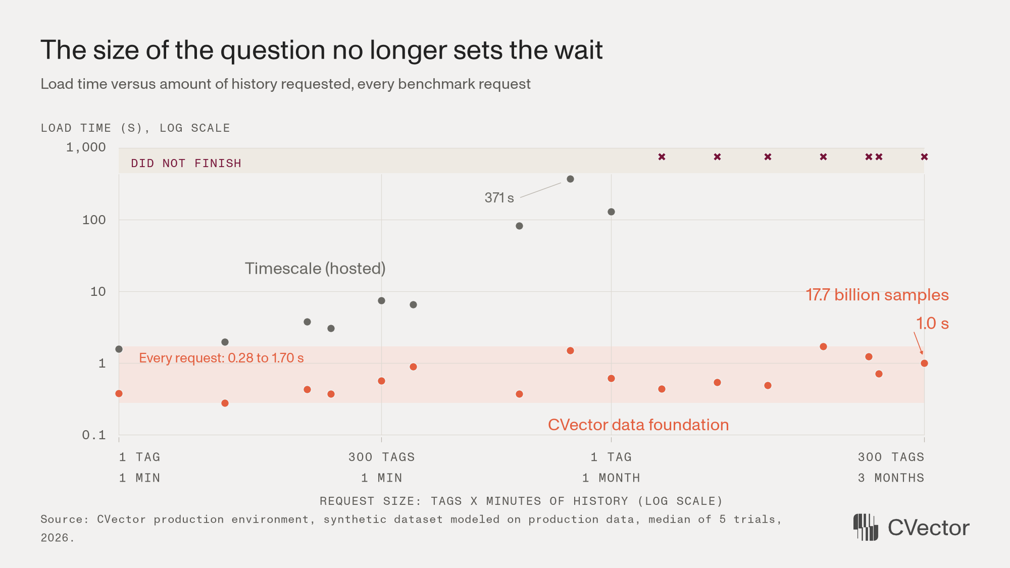
Request size grows tens of millions of times; the data foundation's wait does not.

‍

Matching the tool to the work

Back at the gas plant, agents can now find the hot afternoons, run the cases, and bring the planner the effect on margin and schedule, with the evidence attached. The planner still decides, now while there is time to act.

‍

The principle we follow is: when one input becomes cheap, the limit moves to the next, and a tool that was good enough becomes the constraint. So match the tool to the shape of the work.

‍

We believe the best industrial AI platforms of the next generation will be built on the best data foundations, holding not only time-series data but also the knowledge, context, and tools that agents rely on.

‍

With this data foundation, every price swing, drifting tag, and stale LP yield becomes margin captured instead of margin missed. Agents rerun what-if cases with every power price update, check every tag against years of history around the clock, and recalibrate LP models every day.

‍

Running a site with years of history? Running agents for industrial plants? Curious how CVector's data foundation works? Reach out at info@cvector.com. Let's compare notes and dive into the raw benchmark data together.